Lattice-Boltzmann Methods

The Lattice-Boltzmann method (LBM) method is a way of solving complex flows based on a kinetic description of the fluid through the particles distribution function. This is in contrast to most fluid solvers that instead evolve the macroscopic fluid variables (density, velocity, pressure). It is essentially a description of the mesoscopic scales in a fluid, far above the scales of particle-particle interactions, and thus shares many similarities with the theory of kinetic plasmas. Lattice-Boltzmann methods have proven to be flexible and highly parallelizable, which makes them a very attractive numerical method compared to Finite-Volume methods.

The starting point of a LB method is the kinetic Boltzmann equation that describes the time evolution of the particle distribution function $f (x,v,t)$ in coordinate space and velocity space due to external forces and collisions:

$$ \frac{\partial f}{\partial t} + v\frac{\partial f}{\partial x} + \dot{v}\frac{\partial f}{\partial v} = \Omega(f), $$

where $\Omega(f)$ is a collision operator that represents thermodynamic relaxation towards an equilibrium function. In plasma physics, the Boltzmann equation is coupled to the Maxwell equations for the electromagnetic fields that enter in the acceleration term $\dot{v}$.

The key to the discrete form of the Lattice-Boltzmann equation is to discretize the velocity variable on a lattice with given directions $c_i$. This is done by performing a moment expansion in terms of the Hermite polynomials, and discretizing the resulting integrals over the velocity. The discrete-velocity Boltzmann equation then reads (neglecting the force term for simplicity):

$$ \frac{\partial f_i}{\partial t} + c_{i\alpha}\frac{\partial f}{\partial x_{\alpha}} = \Omega(f_i), $$

where $f_i$ is the value of the distribution function on the i-th lattice vector. Discretizing in time and using the methods of characteristics the solution of $f_i$ can be written as:

$$ f_i (\mathbf{x} + \mathbf{c}_i \Delta t, t+\Delta t) = f_i (\mathbf{x}, t) + \Delta t \Omega (f_i). $$

The macroscopic fluid variable are then computed as velocity moments of the distribution function, i.e.:

$$ \begin{align*} \rho (\mathbf{x},t) = \sum_i f_i (\mathbf{x},t), \end{align*} $$ $$ \begin{align*} \rho (\mathbf{x},t) \mathbf{u} (\mathbf{x},t) = \sum_i \mathbf{c}_i f_i (\mathbf{x},t). \end{align*} $$

cuLBM

The elegance of the LBM and its strong connections to plasma physics got me very interested, and so I decided to study LBM more in depth and code my own 2D solver in Python, using numba and cupy libraries to offload the computations to GPUs.

The code is a playground for further development, and I plan to progressively implement more complicated models as I go along. It is called cuLBM and publicly available on GitHub.

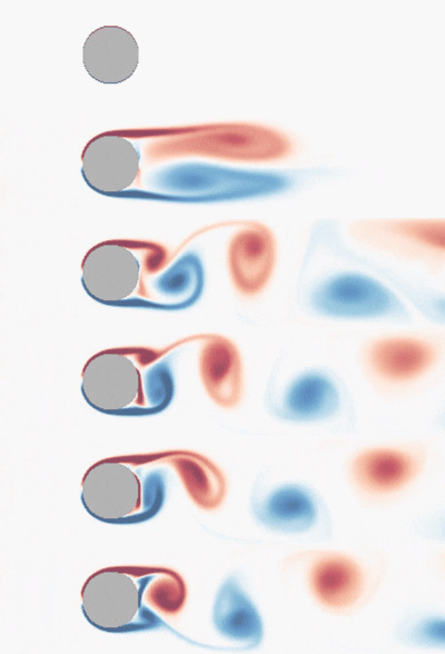
Here is a short demo of a subsonic flow past a cylinder at Reynolds number of $Re=750$, where we can see the development of Karman vortices in the wake of the cylinder.

Features

Currently, cuLBM features:

• (Weakly) compressible D2Q9 discretization of the Navier-Stokes equations (without external forces)
• Runs on NVIDIA GPUs
• Different boundary conditions:
  • wall;
  • inlet, outlet pressure boundary conditions (based on Zou, He 1997);
  • slip;
  • periodic;
  • moving wall with velocity boundary condition (Zou, He 1997);
• Types of obstacles:
  • ellipses (or circles);
  • rectangles;
• Turbulence models:
  • Smagorinsky
• Surface-normal detection for calculations of drag forces on obstacles

Tests and benchmarks

As I implement new features, I also make sure to validate the performance of the code with analytical results or with solutions obtained with different methods. Right now the benchmark tests include:

• Poiseuille flow (0.5% error with respect to theoretical pressure drag)
• Lid-driven cavity (4% max error in comparison with openFOAM)
• Potential flow around a cylinder