Bayesian Regression
In this post I am going to apply Bayesian regression to fit some simulation data that I obtained back in 2022 and attempt to retrieve the theoretical relationship that we proposed in Perrone & Latter 2022 https://doi.org/10.1093/mnras/stac974.
The full Jupyter notebook is available on Codeberg here.
Define the data for the Bayesian regression
The data is taken from Perrone & Latter 2022, Table 1, and represents the outcome of several numerical simulations of the magneto-thermal instability in 2D varying the two main parameters $Pe$ (Peclet number) and $N^2$ (square of the Brunt-Vaisala frequency). The observed data ($K$) represents the kinetic energy at saturation in code units. The std on $K$ is also included for completeness but not used in this notebook.
N2 = np.array([0.1,0.1,0.1,0.1,0.1,0.1,0.05,0.1,0.2,0.4,0.6])
Pe = np.array([6e2,1e3,6e3,1e4,3e4,6e4,3e3,3e3,3e3,3e3,3e3])

K = np.array([1.94e-3, 1.17e-3, 1.93e-4, 1.16e-4, 3.63e-5,
     1.74e-5, 7.26e-4, 3.91e-4, 2.08e-4, 1.04e-4,
     6.80e-5])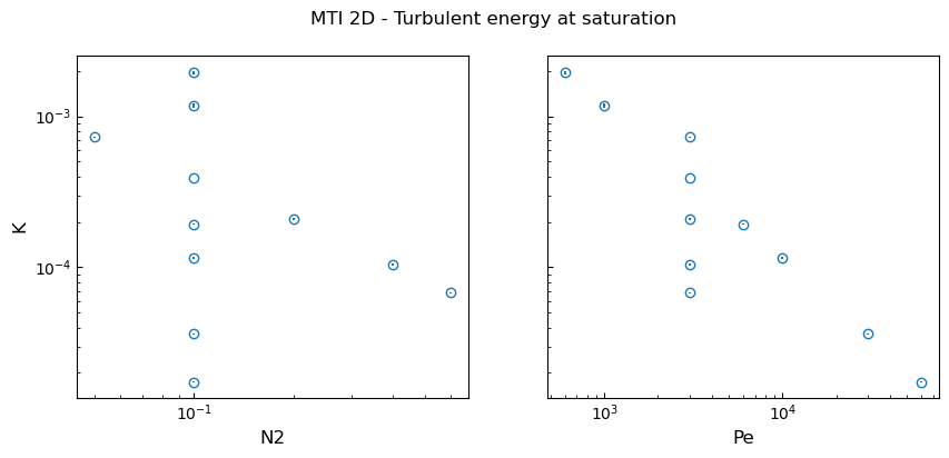
Definition of the models
We define two models for the relationship between $K$ and $N^2$, $Pe$.
1. The first represents a simple power law of the form $K = a \cdot (N^2)^{b1} (Pe)^{b2}$, with $a$, $b1$ and $b2$ unknown parameters. This model can be easily transformed into a linear regression by taking the log of both sides, but we will keep it in this form here for comparison purposes.
2. The second model represents a variation of the previous equation: $K = a \cdot (N^2)^{b1} \tanh{(Pe)^{b2}}$. Given the data there is not a strong motivation for the $\tanh$, but we use it for comparison.
Note that in Perrone & Latter 2022 we derive a relationship between $K$, $N^2$ and $Pe$ based on an analysis of the energy fluxes between large and small scales. The relationship is found to be $K \sim (N^2)^{-1} Pe^{-1}$.
Bayesian regression and definition of the priors
In Bayesian regression we assume that the observable $K$ is a normally-distributed variable with an expected value that corresponds to that predicted by either model 1 or 2, with variance that represents the observation error. Observational uncertainties on $K$ (e.g. given by noisy data) can be included in the modelling, but we neglect them here for simplicity.
We include information on the parameters of the model $a$, $b1$ and $b2$ in the form of priors, which we take to be normally distributed around some reasonable values.
base_model = pm.Model()

with base_model:

    # Priors for unknown model parameters
    a = pm.Normal("a", mu=0.1, sigma=2)
    b = pm.Normal("b", mu=-1, sigma=2, shape=2)
    sigma = pm.HalfNormal("sigma", sigma=0.1)

    # Expected value of outcome
    mu = a * N2**b[0] * Pe**b[1]

    # Likelihood (sampling distribution) of observations
    likelihood  = pm.Normal("likelihood ", mu=mu, sigma=sigma, observed=K)
Bayes theorem
Having defined our models, we want to obtain estimates for the unknown parameters in the model, given the data available to us. In Bayesian analysis this is the posterior distribution. Defining $\mathbf{X}$ as the 2-dimensional input $(N^2, Pe)$, and $\mathbf{b} = (a, b1, b2)$ the parameter vector the posterior $p(\mathbf{b}|K,\mathbf{X})$ is given by the likelihood of the observed data given the inputs and the model $p(K|\mathbf{b},\mathbf{X})$, times the prior for the model parameters $p(\mathbf{b}|\mathbf{X})$, divided by the evidence $p(K|\mathbf{X})$: $$ p(\mathbf{b}|K,\mathbf{X}) = \frac{p(K|\mathbf{b},\mathbf{X}) p(\mathbf{b}|\mathbf{X})}{p(K|\mathbf{X})}. $$
We can sample the posterior (what we are interested in) via various techniques, such as Markov Chain Monte Carlo (MCMC), which can be done by PyMC as follows:
with base_model:
    # draw 500 posterior samples
    trace = pm.sample(500, return_inferencedata=True, tune=1000, idata_kwargs={"log_likelihood": True})
Results of the sampling
With Bayesian regression we can obtain not only the value of the parameters that best fit the model, but we have access to the full probability distribution of said parameters, which we can plot easily with the arviz package:
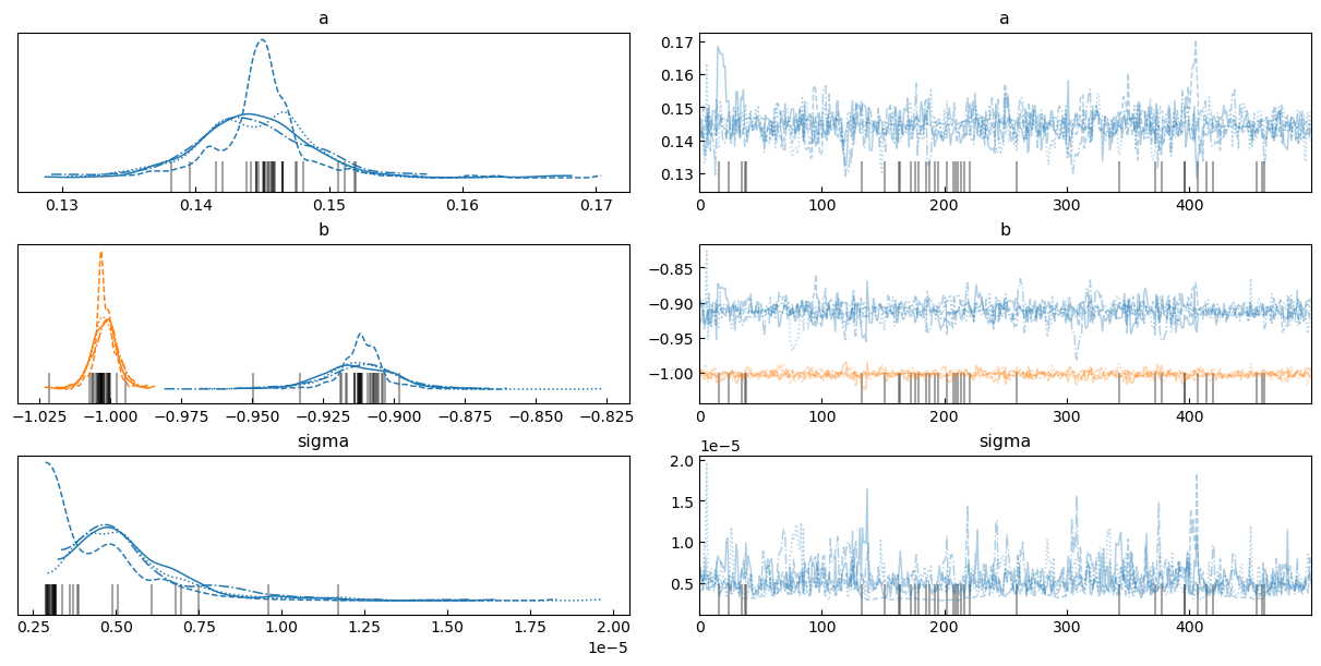
Or in table format:
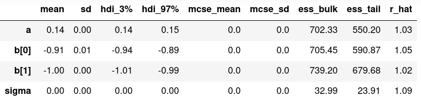
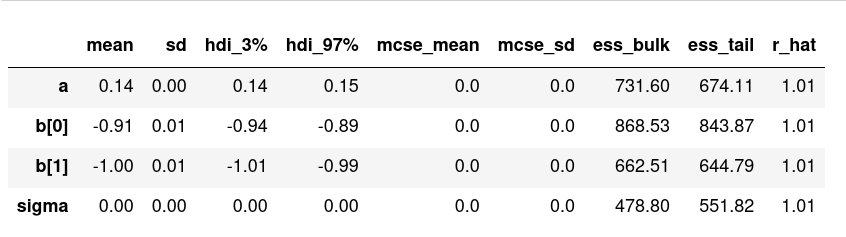
Comparison of the two models
It may seem surprising but both models give in fact very similar results in terms of the parameters $a$, $b1$ and $b2$! In particular $b1$ and $b2$ are very close to what we derived in Perrone & Latter 2022 on theoretical grounds ($b1 = b2 = -1$).
One explanation for the similar performance of the two models is that in the regime explored in the simulations $Pe \gg 1$ the argument of the $\tanh$ in model 2 is very small, and to first order $\tanh (Pe^{b2}) = \tanh (Pe^{-1.00}) \simeq Pe^{-1.00}$, where we Taylor-expanded around zero. As a result, the two models can theoretically both fit the data available to us.
Bayesian regression allows us to compare different models for the same data in a more systematic manner by comparing their log-likelihoods, where the likelihood is the same that we defined before $p(K|\mathbf{b},\mathbf{X})$, which represents the likelihood of the observed data given the inputs and the model. The higher the likelihood, the better fit is the model to the data. It is important to notice that the likelihood is meaningful only in relative terms compared to other models. Its magnitude individually does not mean much.
The log-likelihood was sampled by default during the sampling procedure, so we can access it directly and compare the two models in the following table:

From the table above, we can see that the base model has only a slightly higher log-likelihood than the alternative model (in fact depending on the MCMC sampling the results might change), which in this case does not allow us to draw definitive conclusions (as mentioned earlier, for the parameters explored in the simulations the two models behave very similarly). Nevertheless, we managed to obtain a very good fit to the theoretical model using Bayesian regression!