Recently I have been learning how to apply autodifferentiation in JAX to the study of various physical systems, such as the Lorenz system, which is possibly the most famous example of chaotic dynamics arising from nonlinear deterministic equations.

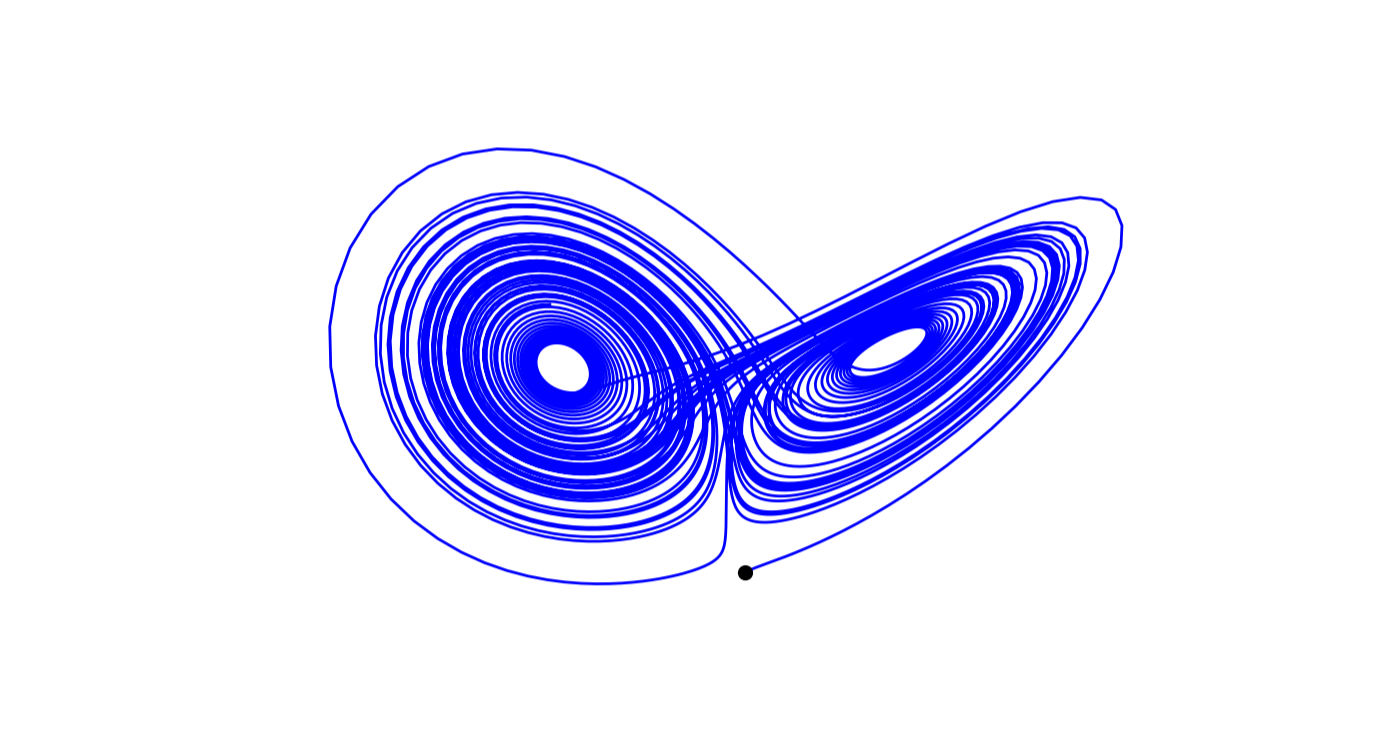
More precisely, the Lorenz system is a set of 3 equations that was derived to describe atmospheric convection (one equation for the velocity field, $X$, and 2 equations for the temperature fluctuation, $Y$ and $Z$ in the original naming). For certain combinations of parameters it gives rise to beautiful butterfly-shaped trajectories that diverge exponentially with time.

One nifty application is the estimation of the Lyapunov exponent of the Lorenz system by propagating the value of a small perturbation during the trajectory using the Jacobian matrix of the system, which is easily done in JAX.

Inspired by the excellent series on the Lorenz sytem in JAX (https://www.youtube.com/playlist?list=PLISXH-iEM4JmYt5GYfitw_EjFu6_zAo26) I thought it would be cool to go one step further and use JAX to try to map the phase-space of the parameters that allow chaotic orbits and those that do not (TL;DR: lots of jax.vmap were used).

The three parameters are $\sigma$, $\rho$, $\beta$, (related to viscosity, temperature difference and thermal diffusion), with the values $\sigma=10$, $\rho=28$ and $\beta=8/3$ giving rise to chaotic dynamics (they are not the only ones however!).

In particular I am interested in the value of the largest Lyapunov exponent: if this is greater than zero, then close orbits will exponentially diverge.

I tracked the Lyapunov of many different combination of parameters (~700) tracked for 5000 timesteps, and for each of them I averaged over 20 different trajectories with random initialization and a warm-up phase. With JAX configured to use my laptop’s GPU the entire procedure takes less than a couple of seconds!

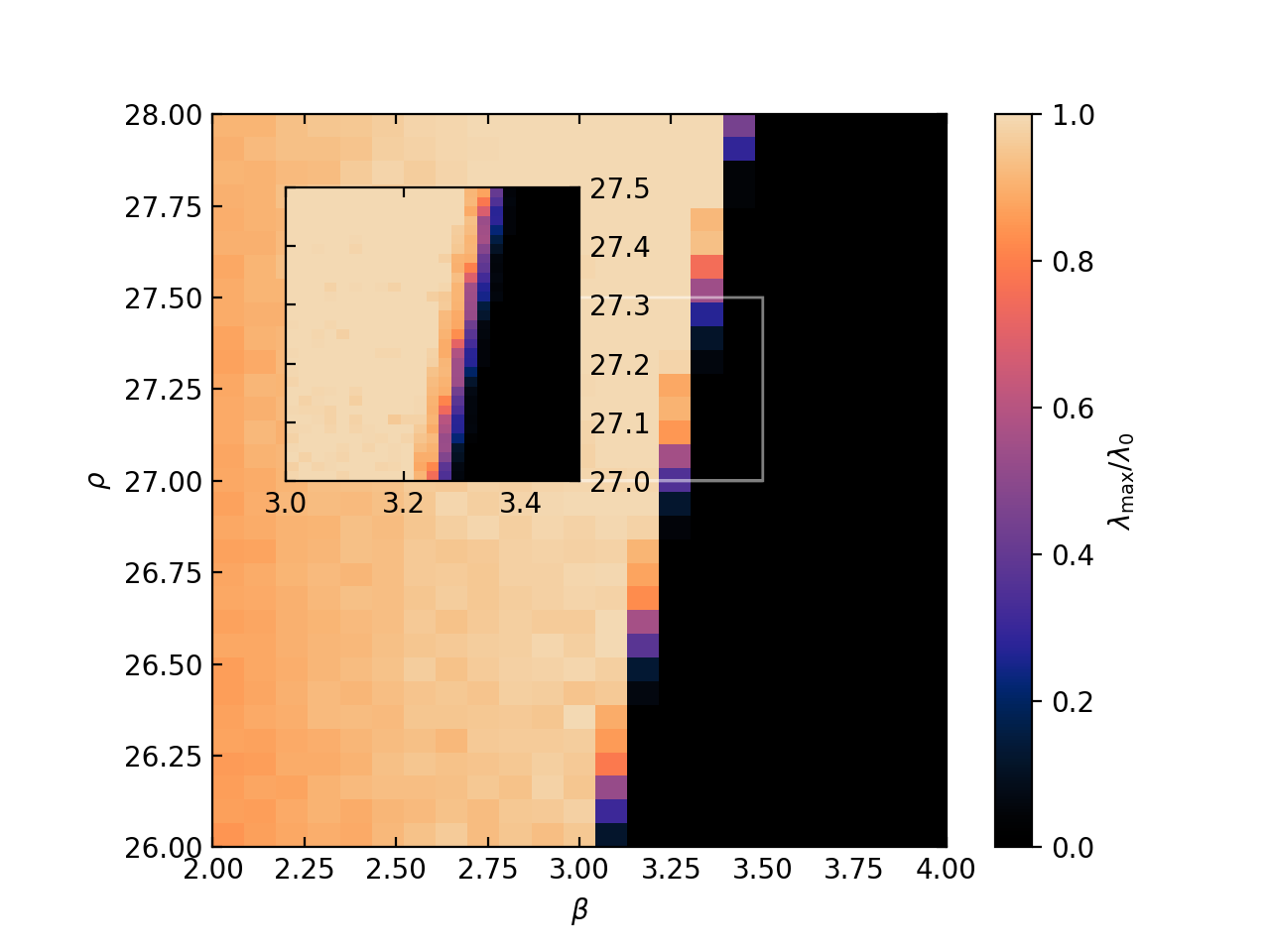
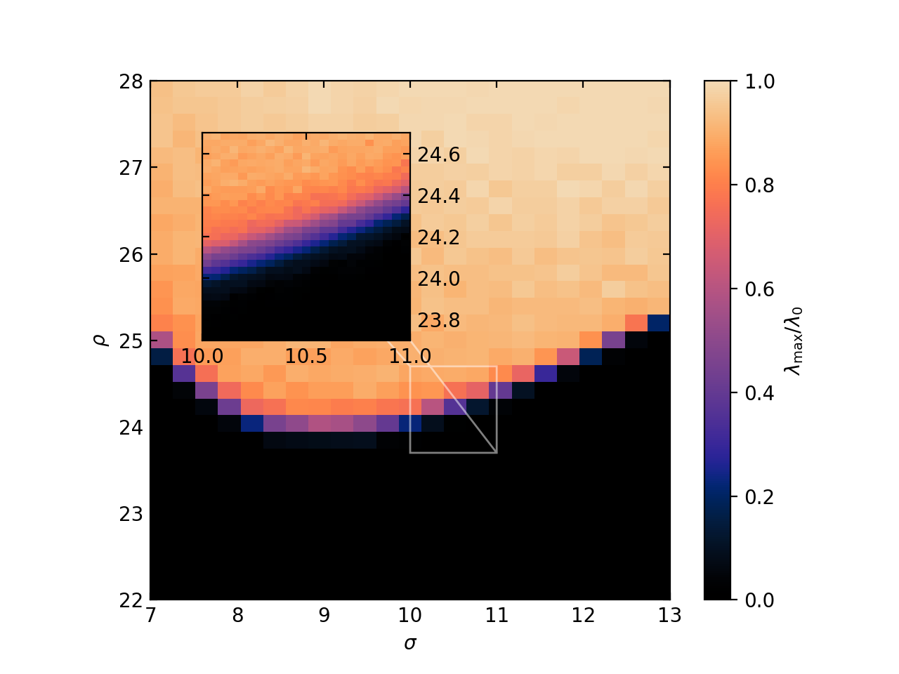
These two plots below show the value of the largest Lyapunov exponent for different parameters, with a zoom-in region. Note the transition around $\rho=24$ (for $\sigma=10$, $\beta=8/3$), which has been derived analytically. It is interesting that there is a quite sharp edge between the regions with chaotic orbits and those without!