I have been learning about Physics-Informed Neural Networks (PINNs), which are a very interesting class of neural networks that can be used to approximate the solution of physical laws that describe, e.g., the evolution in time or space of a fluid, the diffusion of heat and so forth. One advantage compared to traditional numerical methods to solve differential equations is that PINNs do not require uniformly-sampled data points, or regular geometries, and so they can be rather flexible.

One application of PINNs to fluid dynamics is the so-called Helmholtz decomposition of the velocity field $\mathbf{u}$ into two components: a “solenoidal” term $\mathbf{u}_s$ that described vortical motions, and a term $\mathbf{u}_c$ that describes compressive motions. In astrophysical turbulence, compressive and vortical motions can have very different physical effects, for example on particle acceleration, which is why the Helmholtz decomposition is a useful tool.

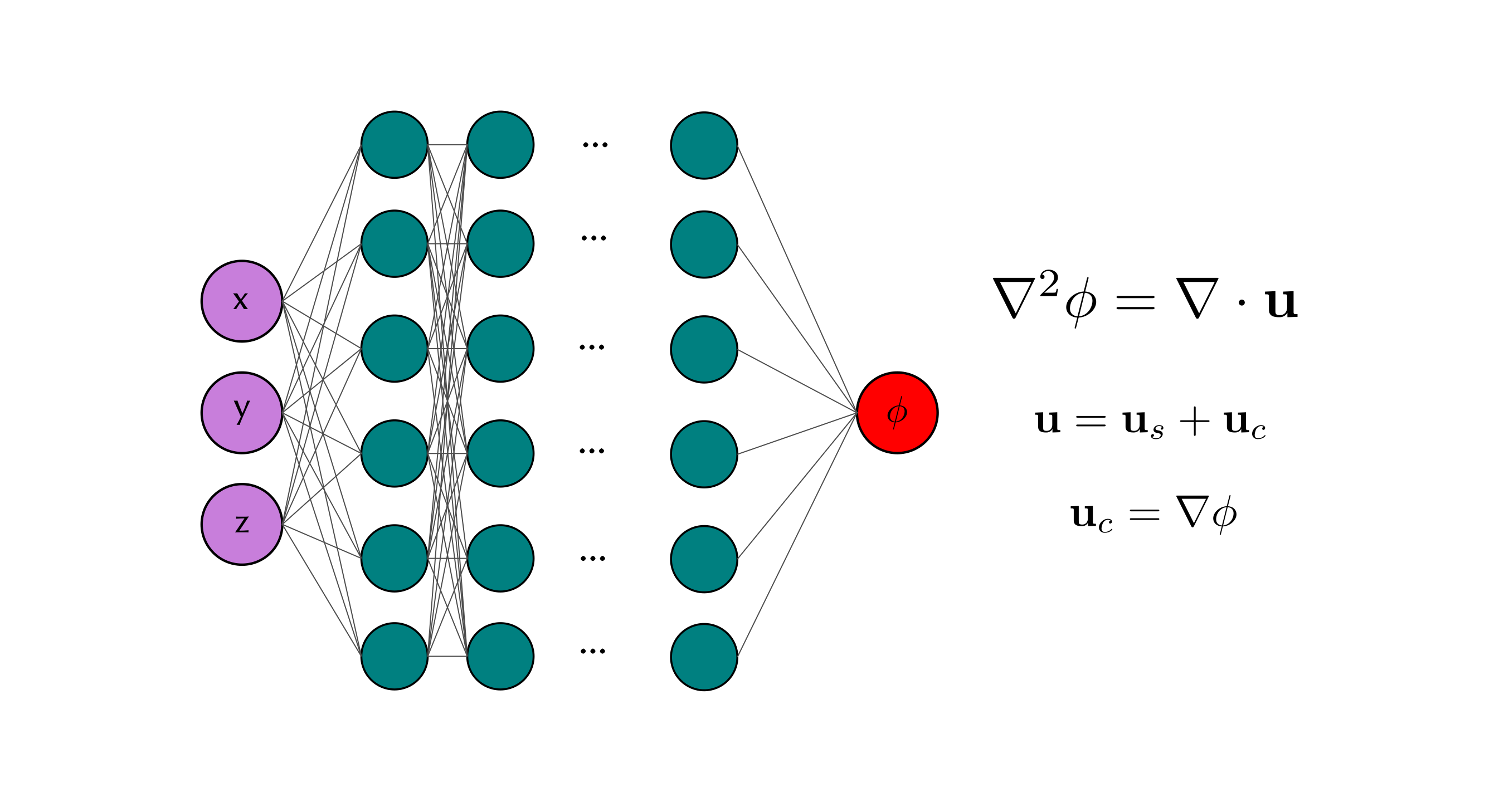
The strategy to separate the velocity in the two components is then as follows: 1. define an auxiliary field $\phi (x,y,z)$ such that $\mathbf{u}_c = \nabla \phi$, where $\nabla$ represents the gradient operator (this is always possible) 2. take the divergence of the velocity and write the equation for $\phi$ as: $$ \nabla^2 \phi = \nabla \cdot \mathbf{u}, $$ which is basically a scalar Poisson equation with the right-hand side known. 3. use the PINN to solve for $\phi$ and thus $\mathbf{u}_c$ 4. obtain the solenoidal field as $\mathbf{u}_s = \mathbf{u} - \nabla \phi$.

So, this is what I will put in practice. Since the following is a testing scenario, I will prescribe a given velocity field (two dimensional for simplicity, although the domain is in 3D) so that we know all the quantities and we can test the performance of the PINN against the ground truth. However, in my work with simulations of astrophysical turbulence the ground truth is not easily accessible, so that scenario is going to be more challenging (but that will be for later).

The architecture of the PINN is in the first instance very simple: a fully-connected multi-layer perceptron with 4 hidden layers, 32 neurons per layer and a sin() activation function. The inputs are the 3-dimensional coordinates x,y,z. The PINN is implemented in JAX, using the libraries Optax and Equinox following the example of this great video. The loss function considers how well the equation in (2.) is satisfied on a set of 500 randomly chosen collocation points (x,y,z) within the domain, and also includes a term to take into account how well the velocity is reconstructed on those same points.

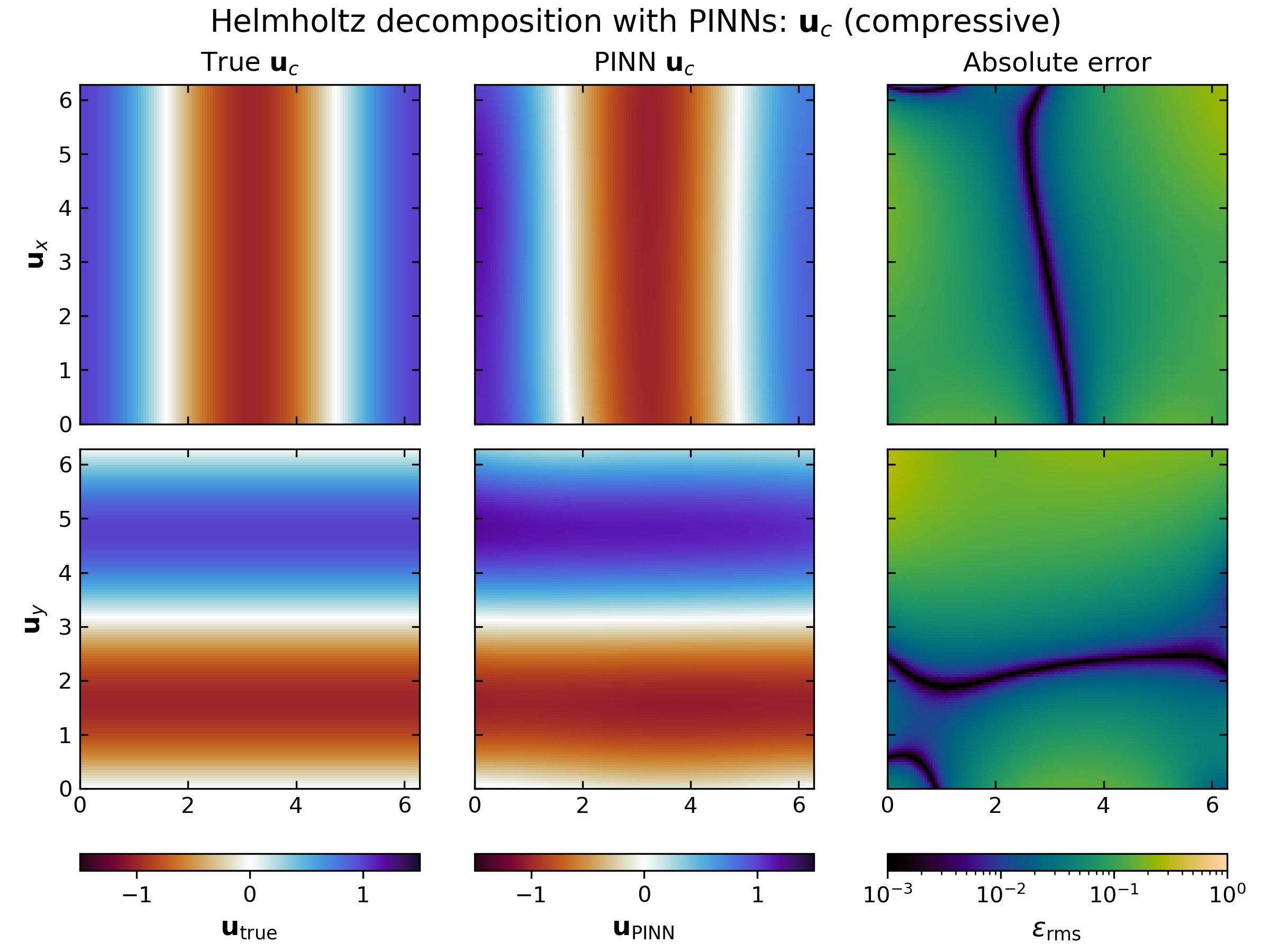
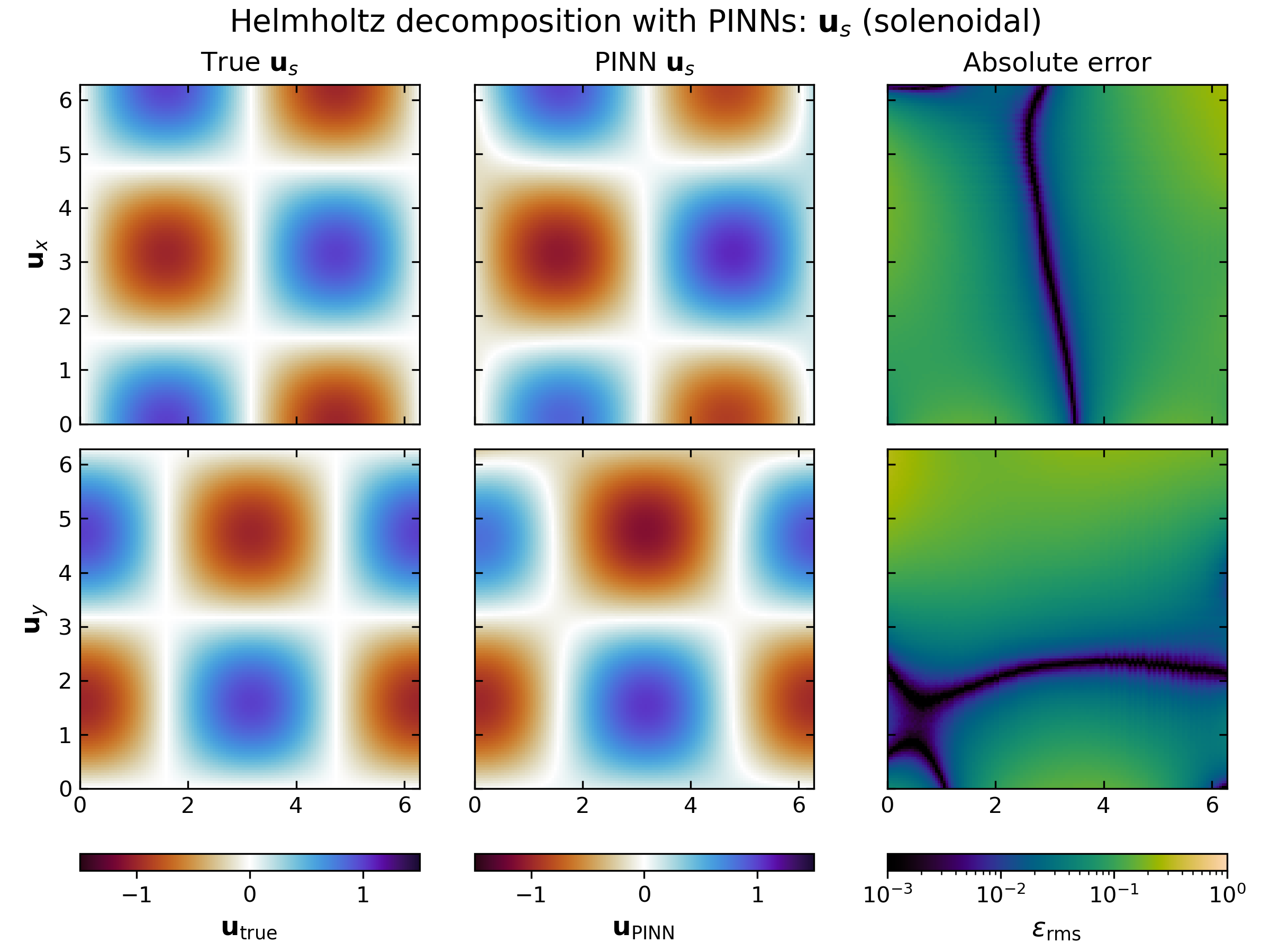
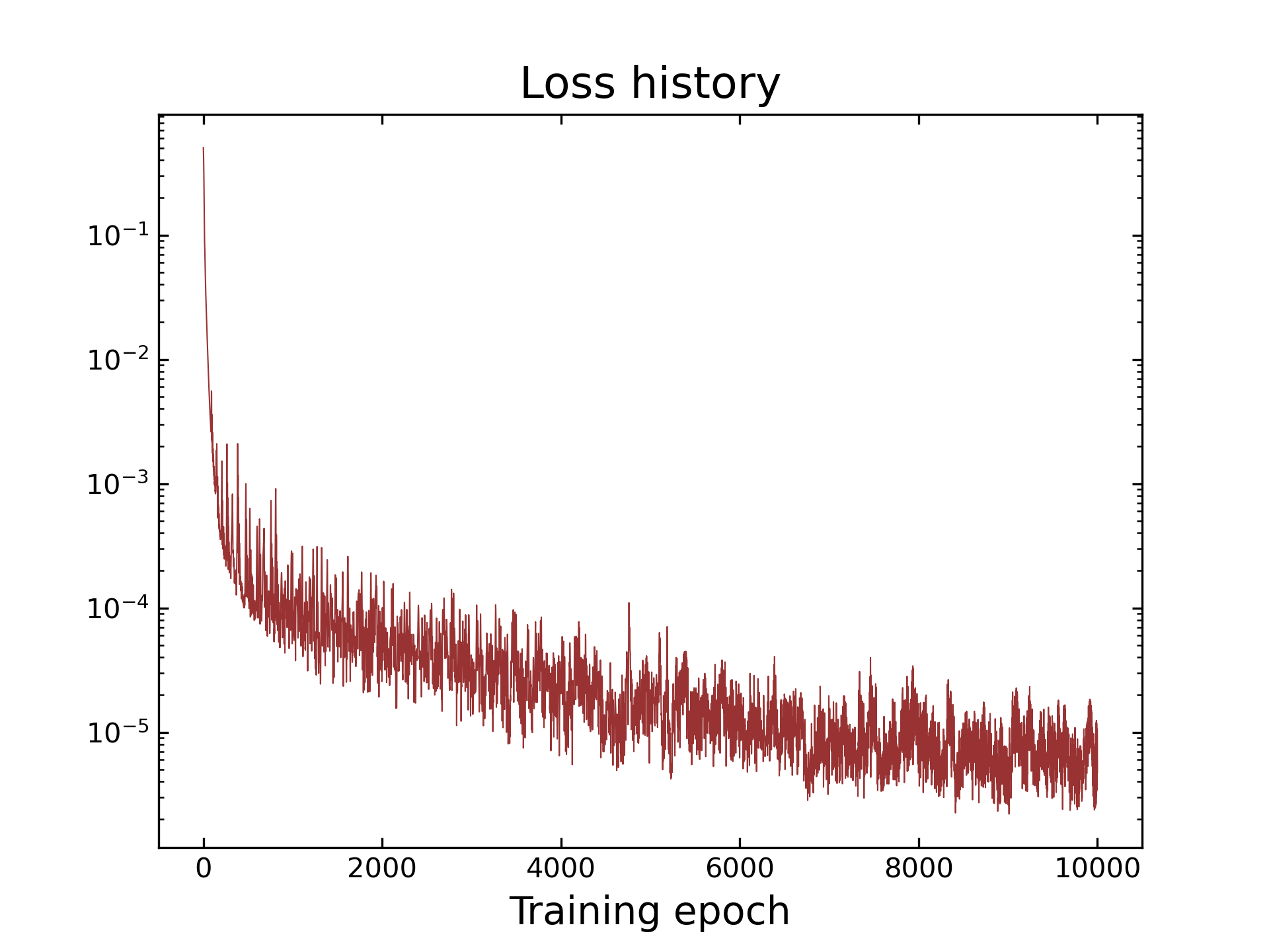
The learning phase is done with a classic Adam optimizer and an exponentially decreasing learning rate. After 10k epochs, the PINN has essentially converged and can be queried to obtain the field $\phi$ and the velocity (using JAX autodiff) on a grid that we can then visualize. The results of this procedure are shown in the two plots below, the first for the compressive velocity $\mathbf{u}_c$ and the second for the solenoidal velocity $\mathbf{u}_s$.

As we can see from the figures, the reconstructed velocity field by the PINN is not perfect, but also not too far off from the ground truth (just a little bent :P), with an rms absolute error of a bit less of 10%. This error can be lowered by increasing the number of the collocation points (e.g. going from 500 -> 1500 points the rms error goes down from 10% to 7%), or by experimenting with different PINNs architecture, which will be the next step!