Physics-Informed Neural Networks (PINNs) can be used in fluid dynamics to perform the so-called Helmholtz decomposition of the velocity field $\mathbf{u}$ into two components: a “solenoidal” term $\mathbf{u}_s$ that described vortical motions, and a term $\mathbf{u}_c$ that describes compressive motions. The basic idea is to use a neural network to solve a Poisson equation where the source is the velocity divergence, and in this way to separate the two velocity components.

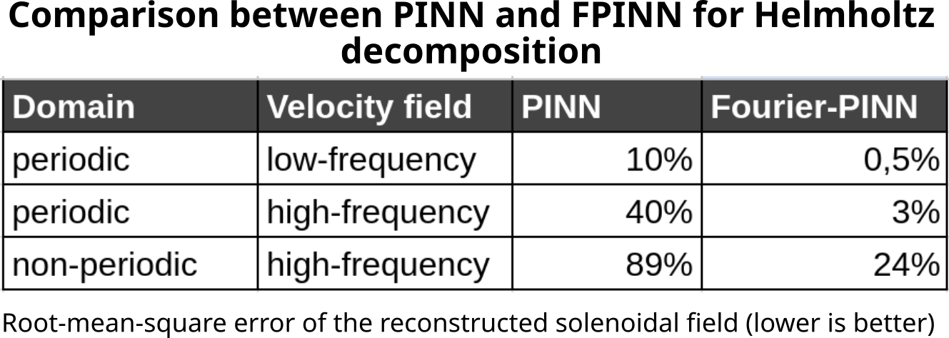
One class of PINNs that has been successfully applied to do the Helmholtz decomposition is the Fourier-PINN, which integrates Fourier features in the neural network itself. If the velocity field is defined on a periodic domain this approach is clearly sensible (and in fact in my tests the rms error decreases by a factor of 10, from 40% to 3%, compared to a classic PINN model!). But what if the domain is non-periodic?

Setup of the problem

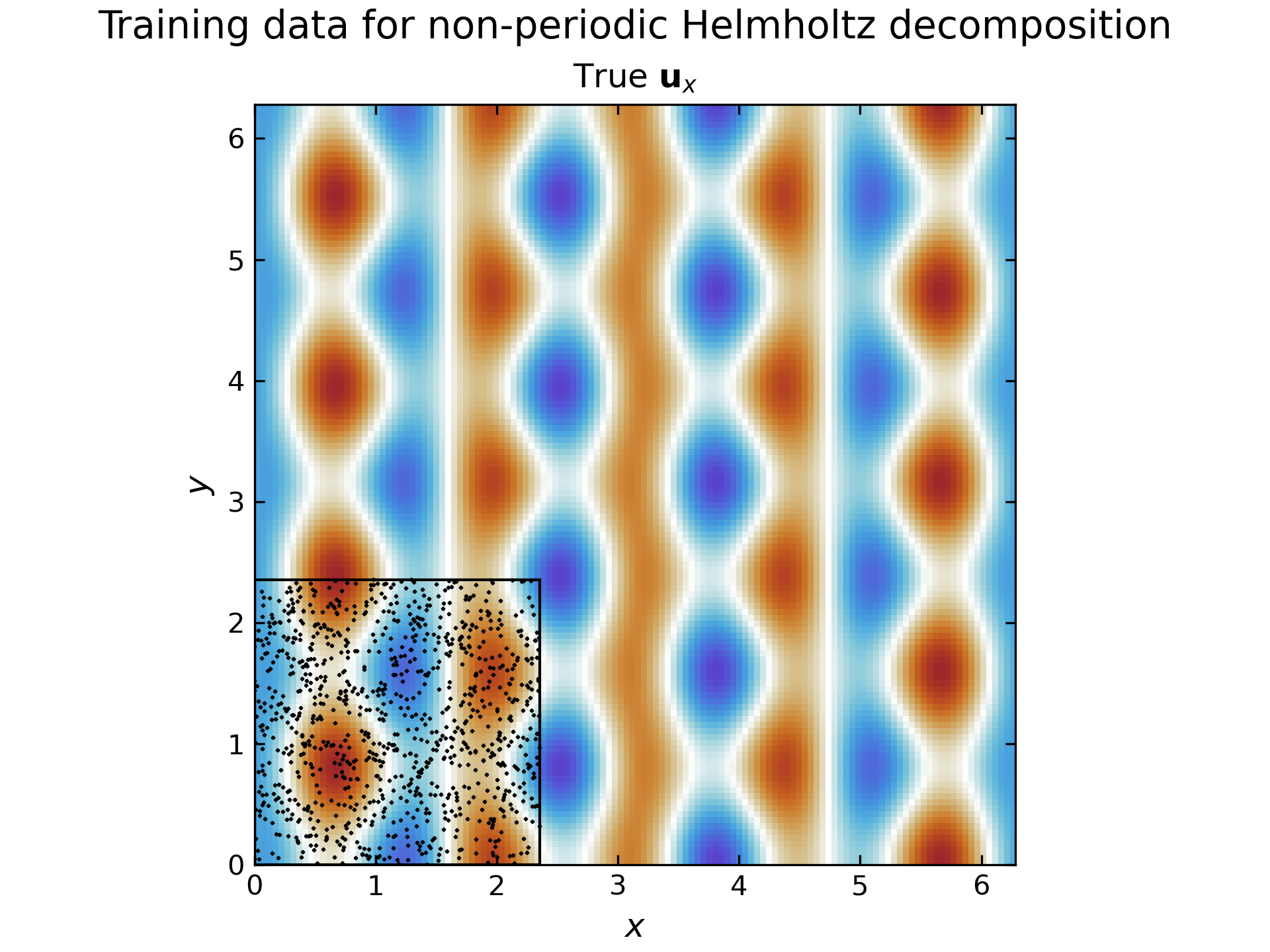
As in the previous test the velocity field is two-dimensional and defined as a superposition of sinusoidal functions, which are easy to work with analytically. The key difference is that I now focus on a sub-portion of the original domain where the velocity field is non-periodic anymore. In practice this means that the network will only train on collocation points that belong in the subdomain.

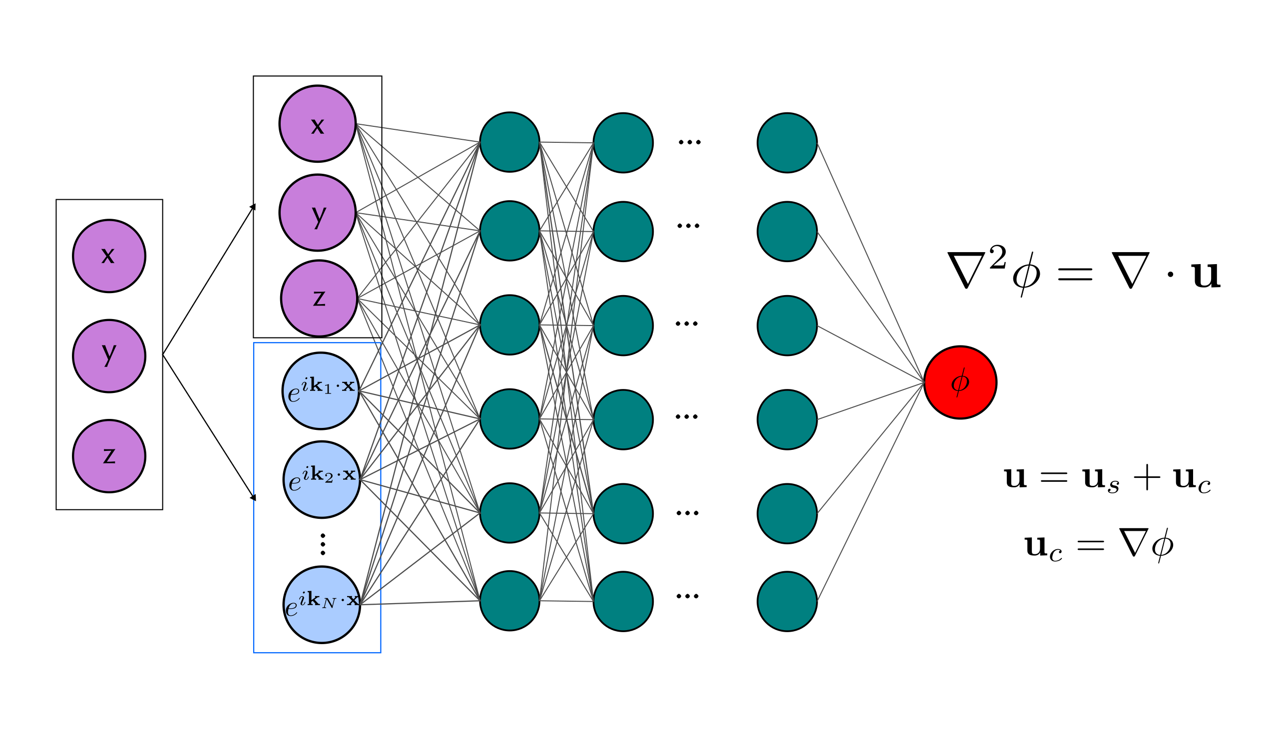
The architecture of the FPINN is very similar to that of the classic PINN: a fully-connected multi-layer perceptron with 4 hidden layers, 32 neurons per layer and a sin() activation function, with inputs the 3-dimensional coordinates x,y,z. However, in the FPINN I now augment the 3 dimensional input by a vector of size N which is made of complex exponentials of the type e^{ik_n x}, where $k_n$ are wave-vectors of choice. The FPINN is implemented in JAX as a subclass of the Equinox.Module class, using N=48 low-frequency Fourier modes.

Finally, the learning phase is done over 20k epochs with a classic Adam optimizer and an exponentially decreasing learning rate.

Results

At the end of the training the PINN has converged and can be queried to obtain the compressive and solenoidal velocities in the subdomain, but can also be used to extrapolate beyond this region to reconstruct the velocity field there.

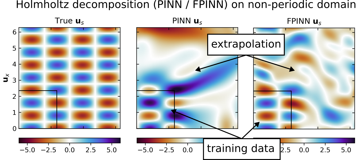
The results are interesting (although I would not call them amazing): the FPINN performs significantly better than the PINN in the non-periodic subdomain (black square in the figure), with an rms error of 24% for the reconstructed solenoidal velocity with the FPINN compared to 89% rms error with the PINN. It’s possible that by increasing the number of collocation points or the Fourier modes in the model the error would decrease, but based on my limited testing this improvement is rather marginal.

Beyond the subdomain, both networks diverge rapidly from the true solution (which is to be expected), although it could be argued that the FPINN performs better in the immediate neighborhood of the subdomain.