Steady-state Navier-Stokes equations with FPINNs

In this experiment I am going to set up a simple Fourier Physics-Informed Neural Network (FPINN, see previous post for details) to solve for the viscous flow past a cylinder using the steady-state incompressible Navier-Stokes equations. This example is deceptively simple because there is no analytical closed solution, making it necessary to solve it numerically by running simulations.

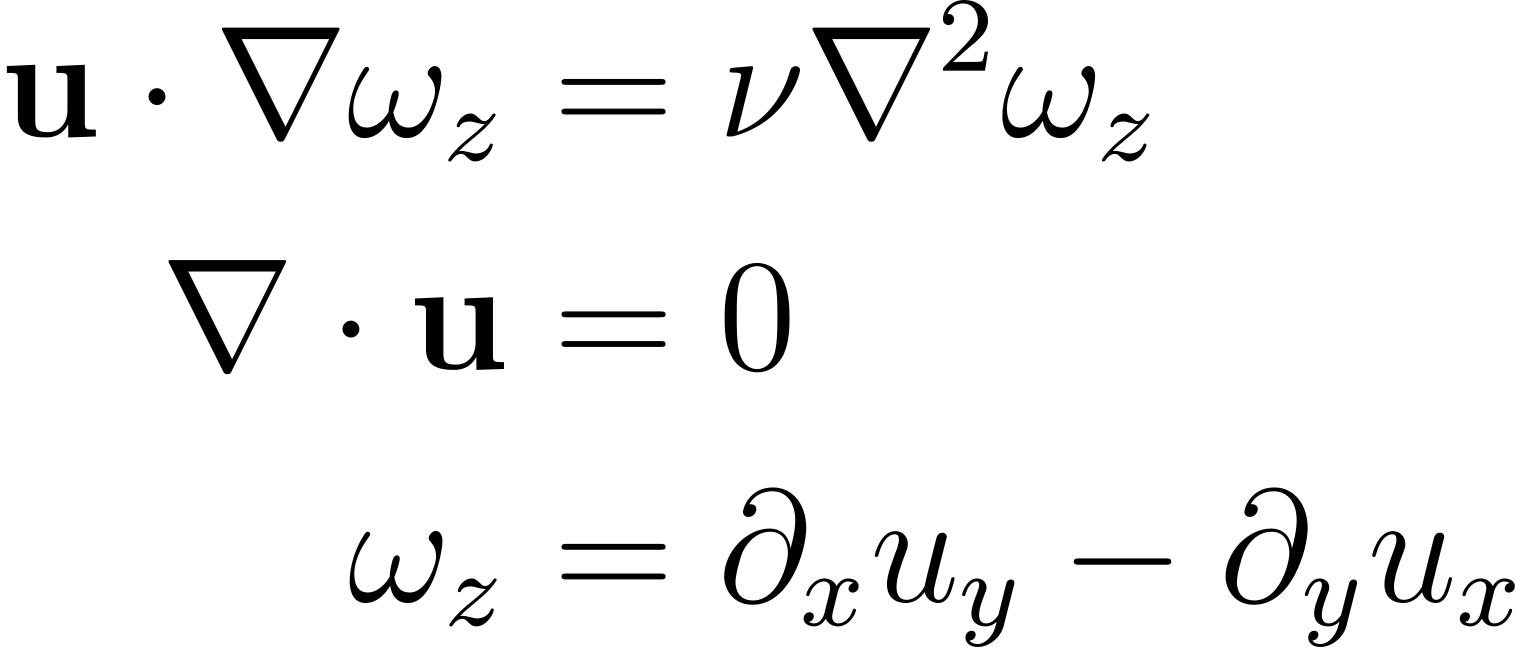
The equations I am trying to solve are as follows (written in vorticity formulation):

The problem is set up as follows:

• the flow is 2D, on a Cartesian mesh with size 1 in both x and y;
• we fix the velocity at the boundaries to be aligned with the x direction and with constant value;
• we set the Reynolds number Re=1;
• the cylinder has a radius R=0.2 and is placed right in the middle of the domain;
• the velocity on the cylinder is set to zero in both components (no-slip boundary condition)

Here is an example of a simulation using a Lattice-Boltzmann code I wrote myself:

Architecture of the FPINN

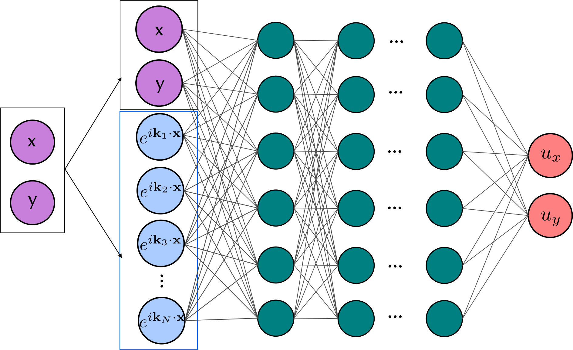
The FPINN used here is a simple network made of a fully-connected multi-layer perceptron with 4 hidden layers, 32 neurons per layer and a sin() activation function, with inputs the 2-dimensional coordinates x,y, which are then augmented by a vector of size N which is made of complex exponentials of the type e^{ik_n x}, where $k_n$ are wave-vectors of choice. The FPINN is implemented in JAX as a subclass of the Equinox.Module class, using N=24 low-frequency Fourier modes.

The learning phase is done over 20k epochs with a classic Adam optimizer and an exponentially decreasing learning rate. The loss function is particularly important and consists of different pieces:

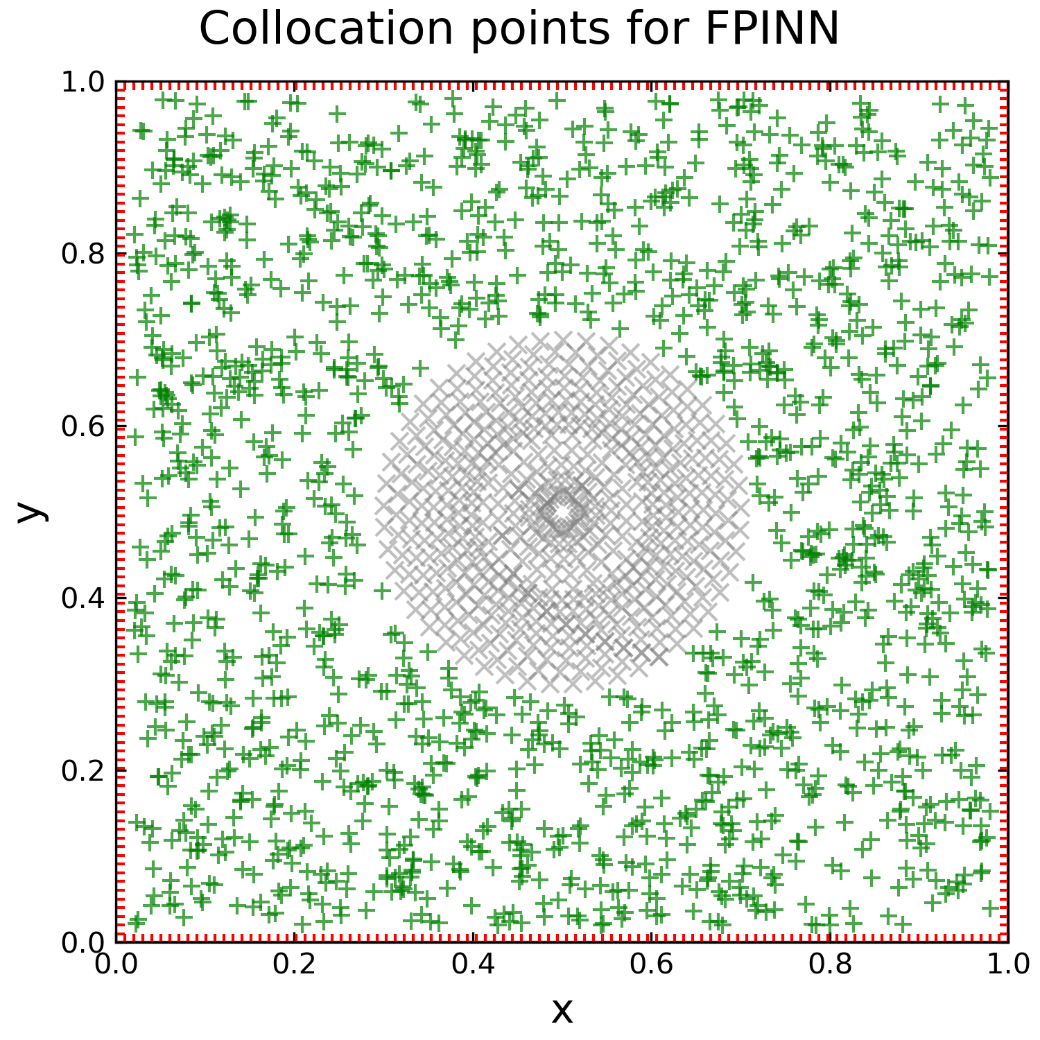
1. the loss related to the solution of the vorticity equation and the incompressibility condition in the inside of the domain on a set of 2000 randomly selected points (gray crossed in the figure);
2. a loss term related to the boundary conditions (left, right, top, bottom) where u_x is set to 1 while u_y is zero (red crosses)
3. a term related to the cylinder (both inside and on its surface) where we require the velocity to be identically zero (gray croses)

Training

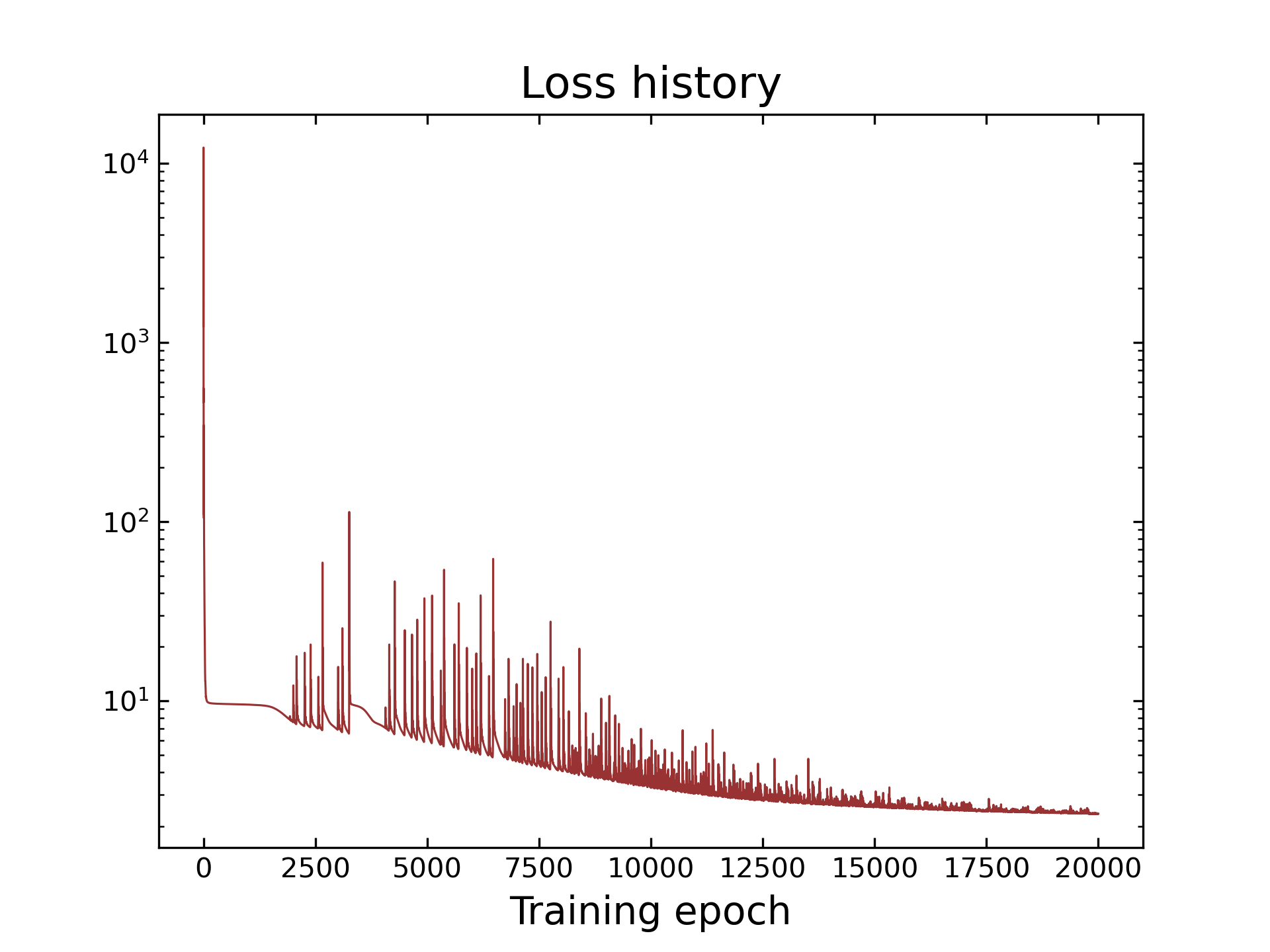
During the training phase I query the PINN to obtain the x and y velocities over the domain, which are shown in the video below. The result at the end of the training is qualitatively very similar to the solution obtained with the Lattice-Boltzmann code, but the match is not perfect. In particular, one can see some funny swirls “inside” the cylinder (where there should be no flow!), and the fact that the y-component of the velocity is about a factor of 2 lower than in the LB simulation, which is made to satisfy the boundary conditions exactly.